appendix
TEMPERATURE G_ 1 – 5
5
DATA SOURCE
5_1 -65.000.000 -> -20.000 [g01]
[-65.000.000 -> 1950]
data source:
The Royal Society, 2013, Climate sensitivity, sea level and atmospheric carbon dioxide, Phil Trans R Soc A 371: 20120294
Hansen J, Sato M, Russell G, Kharecha P. 2013,.
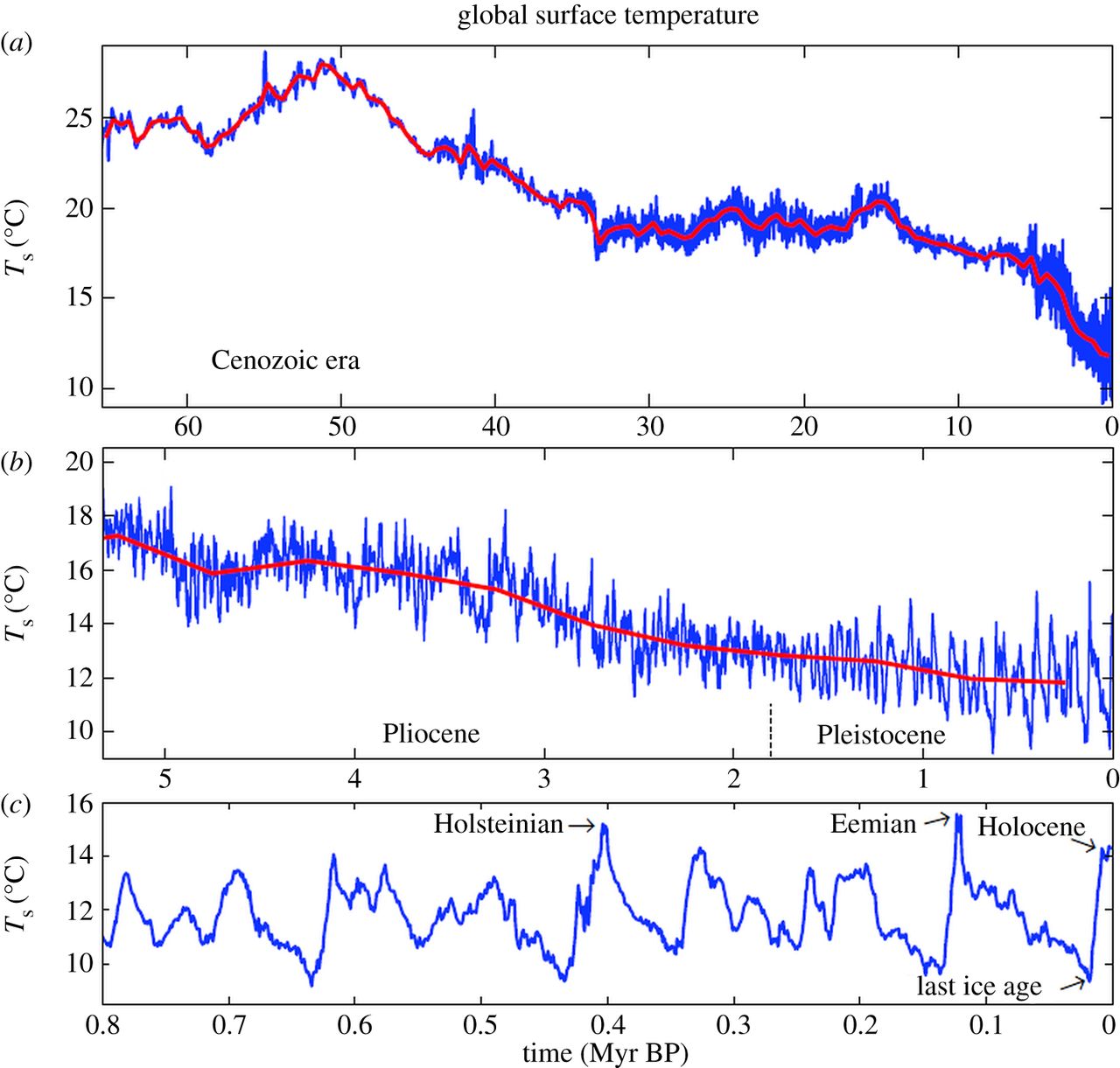
Surface temperature estimate for the past 65.5 Myr
Fig. 4
data source:
The Royal Society, 2013, Climate sensitivity, sea level and atmospheric carbon dioxide, Phil Trans R Soc A 371: 20120294
Hansen J, Sato M, Russell G, Kharecha P. 2013,.
Surface temperature estimate for the past 65.5 Myr
Fig. 4
(a–c) Surface temperature estimate for the past 65.5 Myr, including an expanded time scale for
(b) the Pliocene and Pleistocene and
(c) the past 800. 000 years.
(b) the Pliocene and Pleistocene and
(c) the past 800. 000 years.
PDF_PAPER_http://rsta.royalsocietypublishing.org/content/roypta/371/2001/20120294.full.pdf
PAPER_http://rsta.royalsocietypublishing.org/content/371/2001/20120294
PAPER_http://rsta.royalsocietypublishing.org/content/371/2001/20120294
graph_[-14dC_↓/ x=0 ]_X
5_2_1 -20.000 -> -9.000 [g02]
[-20.000 -> 2100]
data source::
Marcott et al., Science 2013
Science 08 Mar 2013: Vol. 339, Issue 6124, pp. 1198-1201, DOI: 10.1126/science.1228026
A Reconstruction of Regional and Global Temperature for the Past 11,300 Years
credit graph: Jos Hagelaars
Fig. 4
data source::
Marcott et al., Science 2013
Science 08 Mar 2013: Vol. 339, Issue 6124, pp. 1198-1201, DOI: 10.1126/science.1228026
A Reconstruction of Regional and Global Temperature for the Past 11,300 Years
credit graph: Jos Hagelaars
Fig. 4
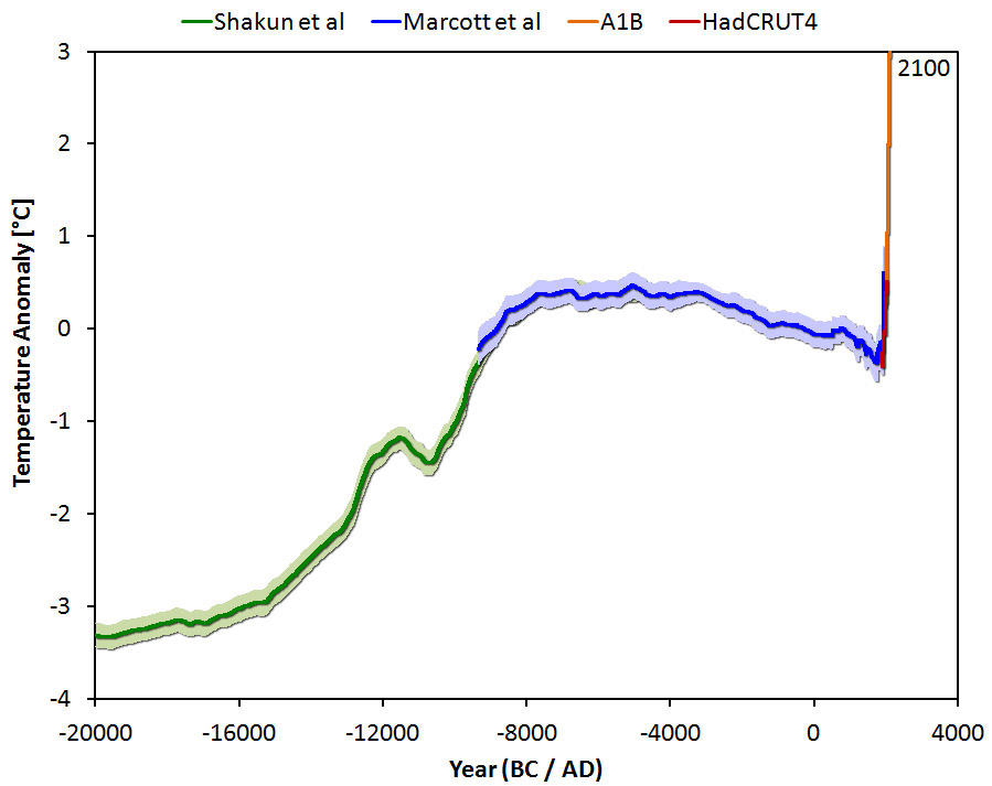
The temperature reconstruction of Shakun et al (green – shifted manually by 0.25 degrees) , of Marcott et al (blue), combined with the instrumental period data from HadCRUT4 (red) and the model average of IPCC projections for the A1B scenario up to 2100 (orange).
Because of the above-mentioned limitations of sediment cores, the new reconstruction does not reach the present but only goes to 1940.
Marcott“ By 2100, global average temperatures will probably be 5 to 12 standard deviations above the Holocene temperature mean.“
Because of the above-mentioned limitations of sediment cores, the new reconstruction does not reach the present but only goes to 1940.
Marcott“ By 2100, global average temperatures will probably be 5 to 12 standard deviations above the Holocene temperature mean.“
SITE_http://www.realclimate.org/index.php/archives/2013/09/paleoclimate-the-end-of-the-holocene
PAPER_SCIENCE_http://science.sciencemag.org/content/339/6124/1198
PAPER_SCIENCE_http://science.sciencemag.org/content/339/6124/1198
graph_[+0.2dC_↑/1961-1990 = 0]_B
5_2_2 -9.000 -> 0 [g02]
[-9.000 -> 2000]
data source:
Marcott et al., Science, 2013
Science 08 Mar 2013: Vol. 339, Issue 6124, pp. 1198-1201, DOI: 10.1126/science.1228026
Global temperature reconstruction
credit graph: Graph: Klaus Bitterman
Fig. 1
data source:
Marcott et al., Science, 2013
Science 08 Mar 2013: Vol. 339, Issue 6124, pp. 1198-1201, DOI: 10.1126/science.1228026
Global temperature reconstruction
credit graph: Graph: Klaus Bitterman
Fig. 1
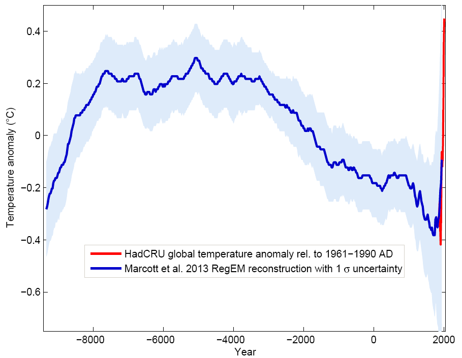
Blue curve: Global temperature reconstruction from proxy data of Marcott et al, Science 2013.
Shown here is the RegEM version – significant differences between the variants with different averaging methods arise only towards the end, where the number of proxy series decreases. This does not matter since the recent temperature evolution is well known from instrumental measurements, shown in red (global temperature from the instrumental HadCRU data).
Shown here is the RegEM version – significant differences between the variants with different averaging methods arise only towards the end, where the number of proxy series decreases. This does not matter since the recent temperature evolution is well known from instrumental measurements, shown in red (global temperature from the instrumental HadCRU data).
SITE_http://www.realclimate.org/index.php/archives/2013/09/paleoclimate-the-end-of-the-holocene/
PAPER_http://science.sciencemag.org/content/339/6124/1198
PAPER_http://science.sciencemag.org/content/339/6124/1198
graph_[+0.2dC_↑/1961-1990 = 0]_B
5_2_3 0 -> 1880 [g02]
[0 -> 2000]
data source:
Marcott et al., Science, 2013
Science 08 Mar 2013: Vol. 339, Issue 6124, pp. 1198-1201, DOI: 10.1126/science.1228026
credit graph: Graph: Klaus Bitterman
Global temperature reconstruction for the last 2000 years
Fig. 3
data source:
Marcott et al., Science, 2013
Science 08 Mar 2013: Vol. 339, Issue 6124, pp. 1198-1201, DOI: 10.1126/science.1228026
credit graph: Graph: Klaus Bitterman
Global temperature reconstruction for the last 2000 years
Fig. 3
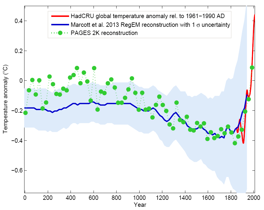
The last two thousand years from Figure 1, in comparison to the PAGES 2k reconstruction (green), which was recently described here in detail.
SITE_http://www.realclimate.org/index.php/archives/2013/09/paleoclimate-the-end-of-the-holocene/
PAPER_http://science.sciencemag.org/content/339/6124/1198
PAPER_http://science.sciencemag.org/content/339/6124/1198
graph_[+0.2dC_↑/1961-1990 = 0]_B
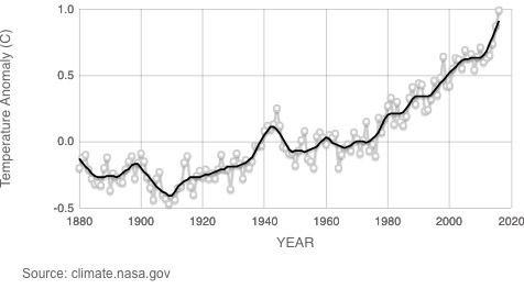
5_3 1880 -> 2016 [g03]
[1880 -> 2016] [0= relative to 1960 -1990 average]
data source:
NASA‘s Goddard Institute for Space Studies (GISS), [2017]
Credit: Credit: NASA/GISS
temperature anomaly [degree celsius]
data source:
NASA‘s Goddard Institute for Space Studies (GISS), [2017]
Credit: Credit: NASA/GISS
temperature anomaly [degree celsius]
black: 5 year mean temperature
grey: annual mean temperature
grey: annual mean temperature
SITE_https://climate.nasa.gov/vital-signs/global-temperature/
DATASET_https://climate.nasa.gov/system/internal_resources/details/original/647_Global_Temperature_Data_File.txt
DATASET_https://climate.nasa.gov/system/internal_resources/details/original/647_Global_Temperature_Data_File.txt
graph_[0dC_↑↓/1951-1980 = 0 ]_A
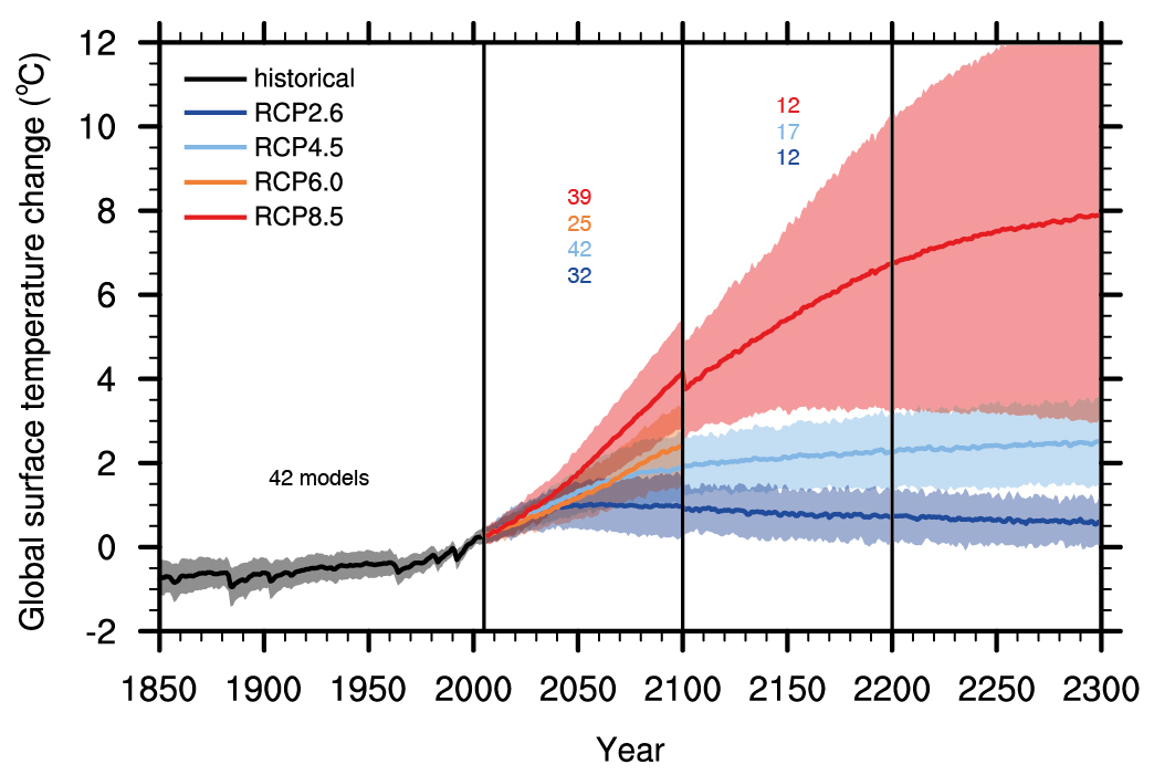
5_4 2016 -> 2300 [g04]
[1765 -> 2300]
[0= relative to 1986 -2005 average = PRE INDUSTRIAL LEVEL]
data source::
IPCC AR5 Fifth Assessment Report_climate change 2013: the physical science basis_chapter 12
Fig. 12.05./page 1054
[0= relative to 1986 -2005 average = PRE INDUSTRIAL LEVEL]
data source::
IPCC AR5 Fifth Assessment Report_climate change 2013: the physical science basis_chapter 12
Fig. 12.05./page 1054
Time series of global annual mean surface air temperature anomalies (relative to 1986–2005) from CMIP5 concentration-driven experiments.
Projections are shown for each RCP for the multi-model mean (solid lines) and the 5 to 95% range (±1.64 standard deviation) across the distribution of individual models (shading).
Discontinuities at 2100 are due to different numbers of models performing the extension runs beyond the 21st century and have no physical meaning. Only one ensemble member is used from each model and numbers in the figure indicate the number of different models contributing to the different time periods. No ranges are given for the RCP6.0 projections beyond 2100 as only two models are available.
PDF_http://www.ipcc.ch/pdf/assessment-report/ar5/wg1/WG1AR5_Chapter12_FINAL.pdf
REPORT_http://www.ipcc.ch/report/ar5/wg1/
PAPER_SPRINGER_https://link.springer.com/article/10.1007/s10584-011-0156-z
IMG_SRC_http://www.ipcc.ch/report/graphics/index.php?t=Assessment Reports&r=AR5 - WG1&f=Chapter 12
REPORT_http://www.ipcc.ch/report/ar5/wg1/
PAPER_SPRINGER_https://link.springer.com/article/10.1007/s10584-011-0156-z
IMG_SRC_http://www.ipcc.ch/report/graphics/index.php?t=Assessment Reports&r=AR5 - WG1&f=Chapter 12
graph_[+4dC_↑/1986-2005 = 0]_C
5
APPEND_DATA SOURCE
5a_1 -500.000.000 -> 0
data source:
J. Veizer et al,Nature, 2000
Credit_GRAP: R. A. Rhode / Wikimedia Commons
summary R.A. Rhode_This figure shows the long-term evolution of oxygen isotope ratios during the Phanerozoic eon as measured in fossils, reported by Veizer et al. (1999), and updated online in 2004.
Such ratios reflect both the local temperature at the site of deposition and global changes associated with the extent of permanent continental glaciation.
As such, relative changes in oxygen isotope ratios can be interpreted as rough changes in climate.
PAPER_http://dx.doi.org/10.1038/35047044
GRAPH_discussion__http://www.realclimate.org/index.php/archives/2014/03/can-we-make-better-graphs-of-global-temperature-history/#ITEM-17010-3
GRAPH_discussion__http://www.realclimate.org/index.php/archives/2014/03/can-we-make-better-graphs-of-global-temperature-history/#ITEM-17010-3

5a_2 GRAPH definition of 0
used "0" in graphs
average of:
1961-1990 = 0_graph_[+0.2dC_↑/]_B
1951-1980 = 0_graph_[ 0dC_↑↓/]_A
1986-2005 = 0_graph_[+4dC_↑/]_C
definition? = 0_graph_[-14dC_↓/ ]_X
average of:
1961-1990 = 0_graph_[+0.2dC_↑/]_B
1951-1980 = 0_graph_[ 0dC_↑↓/]_A
1986-2005 = 0_graph_[+4dC_↑/]_C
definition? = 0_graph_[-14dC_↓/ ]_X
5a_3 variations in the degree SCALE
-800.000 -> _ degree SCALE = 200%
in the graphs
2_2.1 -500.000.000 -> [0]
data source: wikicommons, Glen Fergus
2_5.2 -1000 -> 1999
data source: IPCC AR3, Third Assessment Report_climate change 2001 :the science basis, Fig. 2.22
2_3 -800.000 -> [0]
data source: NASA Jouzel et al. 2007
in the graphs
2_2.1 -500.000.000 -> [0]
data source: wikicommons, Glen Fergus
2_5.2 -1000 -> 1999
data source: IPCC AR3, Third Assessment Report_climate change 2001 :the science basis, Fig. 2.22
2_3 -800.000 -> [0]
data source: NASA Jouzel et al. 2007
4
WHAT IS
4_1 RADIATIVE FORCING
is the difference between enegry that stays on earth [sunligh / insolation absorbed by the Earth] and energy radiated back to space.
Positive radiative forcing means Earth receives more incoming energy from sunlight than it radiates to space.
This net gain of energy will cause warming.
[The amount of radiation reflected by a surface is referred to as its albedo.]
Positive radiative forcing means Earth receives more incoming energy from sunlight than it radiates to space.
This net gain of energy will cause warming.
[The amount of radiation reflected by a surface is referred to as its albedo.]
4_2 CLIMATE SNSITIVITY
data source:
Cambridge University Zero Carbon Society, Stephen Stretton, 2010 0307
Cambridge University Zero Carbon Society, Stephen Stretton, 2010 0307
is the temperature response of the whole climate to a forcing of greenhouse gases.
We know that there are two basic sorts of feedback processes going on in the climate.
Firstly we know that as the
_ temperature rises, relative humidity will stay roughly constant and thus
_absolute humidity will increase.
This leads to more water vapour in the air;
and water vapour is a strong greenhouse gas.
Higher temperatures also has an ambigous (to this author) effect on clouds.
The sum of all these atmospheric effects yields the ‘CHARNEY’ definition of the climate sensitivity which is
the equilibrium temperature rise from a doubling in CO2 concentrations;
assuming that the land albedo and carbon (CO2/Methane) sinks stay constant. (of course they don’t stay constant; we will come to this).
This has been argued to be close to
doubling of CO2 = 0.75°C/(W/m2)*
doubling of CO2 = 4W/m2
doubling of CO2 = 3°C [4 x 0.75]
[*A doubling of CO2 gives an increase in radiative forcing of about 4W/m2,
so multiply the C/(W/m2) by 4 to get the temperature change for doubling CO2]
Hansen et al. (1993) calculated the ice age forcing due to surface albedo change [reflection of energy] to be 3.5 C/(W/m2).
The total surface and atmospheric forcings led Hansen et al. (1993) to infer an equilibrium global climate sensitivity of 3C for doubled CO2 forcing, equivalent to 0.75 +/- 0.25 C/(W/m2).
This empirical climate sensitivity corresponds to the Charney (1979) definition of climate sensitivity, in which ‘fast feedback’ processes are allowed to operate, but long-lived feedbacks are fixed forcings
_Long-lived feedbacks:
atmospheric gases, ice sheet area, land area and vegetation cover are fixed forcings.
_Fast feedbacks include changes of water vapour, clouds, climate-driven aerosols, sea ice and snow cover.
This empirical result for the ‘Charney’ climate sensitivity agrees well with that obtained by climate models (IPCC 2001).
However, the empirical ‘error bar’ is smaller and, unlike the model result, the empirical climate sensitivity certainly incorporates all processes operating in the real world.
speed ot the Fast fedbacks:
50% of the climate response happens in 30 years and the rest takes 1000 years.
So we see in immediate terms (net of the cooling effect of aerosols) about 50% of the climate change that we are likely to see.
[...] Traditionally, ice-melting has been seen as a slow process. But the old models may not be correct; as was shown by record melt rates in the early 21st century.
Paleotological evidence points to times between the ice ages where sea levels have risen metres in a single decade.
Hansen suggests that the relative stability of our epoch may have been to do with the fact that there was a zone of comfort between the melting of the great Eurasian and North American icesheets and the melting of Greenland and West Antarctica
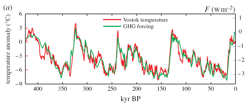
. [...] A cursory inspection of this graph of greenhouse gas forcing shows:
a) A very high correlation (suggesting a strong link between greenhouse gas concentrations and warming)
b) Episodes of very rapid temperature change and ice melt (over the time scale of decades – e.g. the ‘Younger Dryas’ event.)
c) a correlation between the two variables of about 3C/(W/m2)
Now the temperature shifts at the poles by about twice the global temperature change, we can imply a correlation of about 1.5C/(W/m2).
We know that there are two basic sorts of feedback processes going on in the climate.
Firstly we know that as the
_ temperature rises, relative humidity will stay roughly constant and thus
_absolute humidity will increase.
This leads to more water vapour in the air;
and water vapour is a strong greenhouse gas.
Higher temperatures also has an ambigous (to this author) effect on clouds.
The sum of all these atmospheric effects yields the ‘CHARNEY’ definition of the climate sensitivity which is
the equilibrium temperature rise from a doubling in CO2 concentrations;
assuming that the land albedo and carbon (CO2/Methane) sinks stay constant. (of course they don’t stay constant; we will come to this).
This has been argued to be close to
doubling of CO2 = 0.75°C/(W/m2)*
doubling of CO2 = 4W/m2
doubling of CO2 = 3°C [4 x 0.75]
[*A doubling of CO2 gives an increase in radiative forcing of about 4W/m2,
so multiply the C/(W/m2) by 4 to get the temperature change for doubling CO2]
Hansen et al. (1993) calculated the ice age forcing due to surface albedo change [reflection of energy] to be 3.5 C/(W/m2).
The total surface and atmospheric forcings led Hansen et al. (1993) to infer an equilibrium global climate sensitivity of 3C for doubled CO2 forcing, equivalent to 0.75 +/- 0.25 C/(W/m2).
This empirical climate sensitivity corresponds to the Charney (1979) definition of climate sensitivity, in which ‘fast feedback’ processes are allowed to operate, but long-lived feedbacks are fixed forcings
_Long-lived feedbacks:
atmospheric gases, ice sheet area, land area and vegetation cover are fixed forcings.
_Fast feedbacks include changes of water vapour, clouds, climate-driven aerosols, sea ice and snow cover.
This empirical result for the ‘Charney’ climate sensitivity agrees well with that obtained by climate models (IPCC 2001).
However, the empirical ‘error bar’ is smaller and, unlike the model result, the empirical climate sensitivity certainly incorporates all processes operating in the real world.
speed ot the Fast fedbacks:
50% of the climate response happens in 30 years and the rest takes 1000 years.
So we see in immediate terms (net of the cooling effect of aerosols) about 50% of the climate change that we are likely to see.
[...] Traditionally, ice-melting has been seen as a slow process. But the old models may not be correct; as was shown by record melt rates in the early 21st century.
Paleotological evidence points to times between the ice ages where sea levels have risen metres in a single decade.
Hansen suggests that the relative stability of our epoch may have been to do with the fact that there was a zone of comfort between the melting of the great Eurasian and North American icesheets and the melting of Greenland and West Antarctica
. [...] A cursory inspection of this graph of greenhouse gas forcing shows:
a) A very high correlation (suggesting a strong link between greenhouse gas concentrations and warming)
b) Episodes of very rapid temperature change and ice melt (over the time scale of decades – e.g. the ‘Younger Dryas’ event.)
c) a correlation between the two variables of about 3C/(W/m2)
Now the temperature shifts at the poles by about twice the global temperature change, we can imply a correlation of about 1.5C/(W/m2).
4_2_1 climate sensitivity
is the equilibrium temperature change in response to changes of the radiative forcing. [+- w/m2 earth].
Although climate sensitivity is usually used in the context of radiative forcing by carbon dioxide (CO2), it is thought of as a general property of the climate system: the change in surface air temperature (ΔTs) following a unit change in radiative forcing (RF), and thus is expressed in units of °C/(W/m2).
The climate sensitivity specifically due to CO2 is often expressed as the temperature change in °C associated with a doubling of the concentration of carbon dioxide in Earth‘s atmosphere.
4_3_1 ICE CORE measurements
measure past changes in both atmospheric greenhouse gas concentrations and temperature.
The measurement of the gas composition is direct:
trapped in deep ice cores are tiny bubbles of ancient air, which we can extract and analyze using mass spectrometers.
Temperature, in contrast, is not measured directly, but is instead inferred from the isotopic composition of the water molecules released by melting the ice cores.
Water is made up of molecules comprising two atoms of hydrogen and one atom of oxygen (H↓2O).
stable isotopes of interest:
16↑O [8 protons and 8 neutrons] _ 99.76% of O in water
18↑O [8 protons and 10 neutrons]
1↑H [1 proton and 0 neutrons] _ 99.985% of H in water
2↑H [1 proton and 1 neutron] = D [Deuterium]
there is less 18↑O and D during cold periods.
They are both heavier molecules - [more neutrones in comp].
It takes more energy to evaporate the water molecules containing a heavy isotope from the surface of the ocean,
As the moist air is transported polewards and cools, the water molecules containing heavier isotopes are preferentially lost in precipitation.
Both of these processes, known as fractionation, are temperature dependent.
IICE CORE under polarised light Ihttps://de.wikipedia.org/wiki/Eisbohrkern

4_3_2 ice core measurements
It is possible to discern past air temperatures from ice cores. This can be related directly to concentrations of carbon dioxide, methane and other greenhouse gasses preserved in the ice.
gas composition:
Stable isotopes of oxygen (Oxygen [16↑O, 18↑O] and hydrogen [D/H]) are trapped in the ice in ice cores. The stable isotopes are measured in ice through a mass spectrometer.
temperature:
Measuring changing isotopic concentrations of δD and δ18↑O through time in layers through an ice core provides a detailed record of temperature change, going back hundreds of thousands of years.

4_4 Gavin Schmidt_TALK
Nasa / GISS [Goddard Institute for Space Studies]
Director of GISS and Principal Investigator for the GISS ModelE Earth System Model
Director of GISS and Principal Investigator for the GISS ModelE Earth System Model
The emergent patterns of climate change. 2014
CONTEXT_TED [Technology, Entertainment, Design conference]
CONTEXT_TED [Technology, Entertainment, Design conference]
3
AGREEMENT
3_1
PARIS climate agreement
is an agreement within the United Nations Framework Convention on Climate Change (UNFCCC) dealing with greenhouse gas emissions mitigation [Reduzierung], adaptation and finance starting in the year 2020.
signed 04 2016
2017 195 UNFCCC members have signed the agreement [164 ratified it].
The contributions of the individual countries are called: NDCs - nationally determined contributions.
[CO2 emissions 2015: China 29.4%, US 14.3%, EEA 9.8%, India 6.8%, Russia 4.9%, Japan 3.5%, other 31.5%]
ARTICLE 3 requires them to be ambitious. Each further ambition should be more ambitious than the previous one, known as the principle of progression.
The specific climate goals are politically encouraged, rather than legally bound.
3_1_1 AIMS
A. Holding the increase in the global average temperature to well below 2 °C above pre-industrial levels and to pursue efforts to limit the temperature increase to 1.5 °C above pre-industrial levels, recognizing that this would significantly reduce the risks and impacts of climate change;
B. Increasing the ability to adapt to the adverse [nachteilig] impacts of climate change and foster climate resilience [Belastbarkeit] and low greenhouse gas emissions development, in a manner that does not threaten food production;
C. Making finance flows consistent with a pathway towards low greenhouse gas emissions and climate-resilient development.“ Countries furthermore aim to reach „global peaking of greenhouse gas emissions as soon as possible“.
3_1_2 START 2018 [-2025]
The global stocktake will kick off in 2018 with a facilitative dialogue, evaluation in 2025.
[parties will evaluate nearer-term goal and and the long-term goal of achieving net zero emissions after 2050+.]
The negotiators of the Agreement, however, stated that the NDCs and the 2 °C reduction target were insufficient;
instead, a 1.5 °C target is required, noting „with concern that the estimated aggregate greenhouse gas emission levels in 2025 and 2030 resulting from the intended nationally determined contributions do not fall within least-cost 2 °C scenarios but rather lead to a projected level of 55 gigatonnes in 2030“,
and recognizing furthermore „that much greater emission reduction efforts will be required in order to hold the increase in the global average temperature to below 2 °C by reducing emissions to 40 gigatonnes or to 1.5 °C“.
[in the first half of 2016 average temperatures were about 1.3 °C [although not the sustained temperatures over the long term which the Agreement addresses] .
3_2 RCP
Representative Concentration Pathways
greenhouse gas concentration trajectories
greenhouse gas concentration trajectories
PRPs describe a possible range of radiative forcing values.
[Positive radiative forcing: Earth receives more incoming energy from sunlight than it radiates to space.]
[in 2100 relative to pre-industrial values +2.6, +4.5, +6.0, +8.5 W/m2]
[Positive radiative forcing: Earth receives more incoming energy from sunlight than it radiates to space.]
[in 2100 relative to pre-industrial values +2.6, +4.5, +6.0, +8.5 W/m2]
RCP 8.5 [green house gas emissions continue to rise throughout 2100+]
RCP 6 [GHGe peak around 2060]
RCP 4.5 [GHGe peak around 2040]
RCP 2.6 [GHGe peak around 2020]
RCP 6 [GHGe peak around 2060]
RCP 4.5 [GHGe peak around 2040]
RCP 2.6 [GHGe peak around 2020]
3_2_1 RCP_ROADMAP_PAPER
Rockström et al, Science, 2017
A roadmap for rapid decarbonization
Science 24 Mar 2017: Vol. 355, Issue 6331, pp. 1269-1271, DOI: 10.1126/science.aah3443
2017–2020: No-Brainers
2020–2030: Herculean Efforts
2030–2040: Many Breakthroughs
2040–2050: Revise, Reinforce
A roadmap for rapid decarbonization
Science 24 Mar 2017: Vol. 355, Issue 6331, pp. 1269-1271, DOI: 10.1126/science.aah3443
2017–2020: No-Brainers
2020–2030: Herculean Efforts
2030–2040: Many Breakthroughs
2040–2050: Revise, Reinforce
PAPER_hhttp://science.sciencemag.org/content/355/6331/1269
PAPER_PDF_http://www.rescuethatfrog.com/wp-content/uploads/2017/03/Rockstrom-et-al-2017.pdf
PAPER_PDF_http://www.rescuethatfrog.com/wp-content/uploads/2017/03/Rockstrom-et-al-2017.pdf

3_2_1_1 RCP_ ROADMAP_ARTICLE
Scientists made a detailed “roadmap” for meeting the Paris climate goals -It’s eye-opening . vox . 2017 03 24
3_2_2 RCP - ROADMAP_SEI
SEI [Stockholm Environment Institute]
A guide to Representative Concentration Pathways
A guide to Representative Concentration Pathways
RCPs are the latest generation of scenarios that provide input to climate models.
RCP 8.5 [continue to rise 2100+]
. Three times today’s CO2 emissions by 2100
. Rapid increase in methane emissions
. Increased use of croplands and decline in grasland which is driven by an increase in population
. A world population of 12 billion by 2100
. Lower rate of technology development
. Heavy reliance on fossil fuels
. High energy intensity
. No implementation of climate policies
RCP 6 peak 2060
. Heavy reliance on fossil fuels
. Intermediate energy intensity
. Increasing use of croplands and declining grasslands
. Stable methane emissions
. CO2 emissions peak in 2060 at 75%t above today’s levels, then decline to 25% above today
. Heavy reliance on fossil fuels
. Intermediate energy intensity
. Increasing use of croplands and declining grasslands
. Stable methane emissions
. CO2 emissions peak in 2060 at 75%t above today’s levels, then decline to 25% above today
RCP 4.5 peak 2040
. Lower energy intensity
. Strong reforestation programmes
. Decreasing use of croplands due to yield increases and dietary changes
. Stringent climate policies
. Stable methane emissions
. CO2 emissions increase only slightly before decline commences around 2040
. Lower energy intensity
. Strong reforestation programmes
. Decreasing use of croplands due to yield increases and dietary changes
. Stringent climate policies
. Stable methane emissions
. CO2 emissions increase only slightly before decline commences around 2040
RCP 2.6 peak 2020
. Declining use of oil . Low energy intensity . A world population of 9 billion by year 2100
. Use of croplands increase due to bio-energy production
. Less intensive animal husbandry . Methane emissions reduced by 40 %
. CO2 emissions stay at today’s level until 2020, then decline and become negative in 2100
. CO2 concentrations peak around 2020, followed by a modest decline to around 400 ppm by 2100
0
LECTURE / TALK / HEARING
0_1 Martin Persson_LECTURE
Assistant Professor at Physical Resource Theory at Department of Energy & Environment at Chalmers University of Technology
Earth´s Climate and Climate Change . 2014
CONTEXT_Earth´s Climate and Climate Change is a PhD course held at Gothenburg University
CONTEXT_Earth´s Climate and Climate Change is a PhD course held at Gothenburg University
0_2 Stefan Rahmstorf_LECTURE
Stefan Rahmstorf . German oceanographer and climatologist.
Since 2000, Prof.at Potsdam University [Physics of the Oceans].
Ph.D. in oceanography from Victoria University of Wellington.
His work focuses on the role of ocean currents in climate change.
HIs co-founded blog_ www.realclimate.org has been described by Nature as one of the top-5 science blogs in 2006.
CONTEXT_Earth101 is a part of series of lectures given at the University of Iceland
Extreme Weather: What Role Does Global Warming Play? . Stefan Rahmstorf . 2016 05 25. Earth101
Is the Gulf Stream System Slowing?. Stefan Rahmstorf . 2016 05 25 . Earth101
0_3 Robert G. Fovell_23_LECTUREs
University of California, Los Angeles, Professor ofAtmospheric and Oceanic Sciences
Meteorology: An Introduction
to the Wonders of the Weather. 2010
TTC_The Teaching Company, Course 1796
TTC_The Teaching Company, Course 1796
0_4 Richard Wilson_12_LECTUREs
Middlebury College, Ph.D., Dartmouth College
Earth's Changing Climate . 2007
CONTEXT_TTC_The Teaching Company, Course 1219
CONTEXT_TTC_The Teaching Company, Course 1219
0_5 The Scientific process_LECTURE
Nima Arkani-Hamed
(Persian: نیما ارکانی حامد) (born 1972)
is an American-Canadian theoretical physicist of Iranian descent, with interests in high-energy physics, string theory and cosmology.
Arkani-Hamed is now on the faculty at the Institute for Advanced Study in Princeton, New Jersey, and director of The Center for Future High Energy Physics (CFHEP) in China, Beijing. He was formerly a professor at Harvard University and the University of California, Berkeley.
Philosophy of Science ++
2016 07 25 . Cornell University
the strategies the science community uses to achieve to work together on one common goal [over such a long period of time].
The "rules" that define the society of science.
2016 07 25 . Cornell University
the strategies the science community uses to achieve to work together on one common goal [over such a long period of time].
The "rules" that define the society of science.
_there is a TRUTH out there, wit a capital T and we try to find it [06:00]
strategies to most successfully ectract the truth:
_be honest with yourself and with others [11:20]
_it doesn't matter who you are, only the content of your ideas are relevant [12:20]
_In Science we have heros not prophets [Steve Weinberg] [13:50]
_We are never in the posession of the whole truth, and never pretend to have complete certainty [14:30]
_we do the best we can and boldly extrapolate ideas we have most confidence in. [15:00]
_be tolerant to other peoples ideas, keep an open mind[15:40]
_it is necessary to be Intolerant + harshly judgemental of ideas that are not perfectly honest, intelectually lazy [especially your own] [16:40]

2
RE_SOURCES
2_1 ZAMG
The Central Institution for Meteorology and Geodynamics
(German: Zentralanstalt für Meteorologie und Geodynamik, ZAMG)
is the national meteorological and geophysical service of Austria.
(German: Zentralanstalt für Meteorologie und Geodynamik, ZAMG)
is the national meteorological and geophysical service of Austria.
2_1_1 -4.600.000.000 -> 2009
data source:
ZAMG
Credit : ZAMG
Middle Europe, temperature
Credit : ZAMG
Middle Europe, temperature
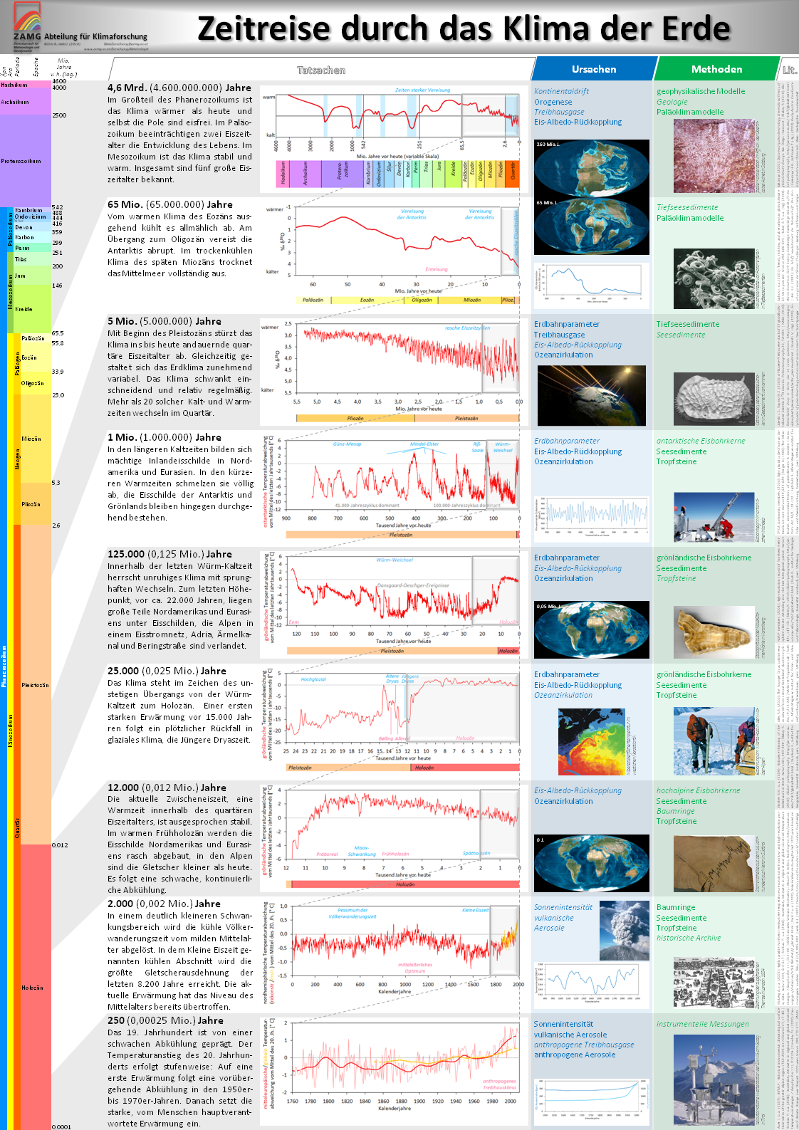
[degree variation in scale]
2_2 NOAA
National Oceanic and Atmospheric Administration
is an American scientific agency within the United States Department of Commerce that focuses on the conditions of the oceans and the atmosphere.
is an American scientific agency within the United States Department of Commerce that focuses on the conditions of the oceans and the atmosphere.
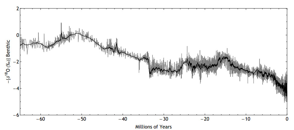
2_2_1 -65.000.000 -> [0]
data source:
NOAA,
math of planet earth
Zachos, J., et al. 2008. Cenozoic Global Deep-Sea Stable Isotope Data. IGBP PAGES/World Data Center for Paleoclimatology Data Contribution Series # 2008-098. NOAA/NCDC Paleoclimatology Program, Boulder CO, USA.
Cenozoic Global Deep-Sea Stable Isotope Data
original data source:
Zachos, J., M. Pagani, L. Sloan, E. Thomas, and K. Billups. 2001. Trends, Rhythms, and Aberrations in Global Climate 65 Ma to Present. Science, Vol. 292, No. 5517, pp. 686-693, 27 April 2001. DOI: 10.1126/science.1059412
The graph has been reconstructed from “proxy data” that are indicators of climate variability and stand-ins for temperature (e.g., isotope ratios in ice cores, fossil pollen, ocean sediments, and coral data).
Because of the diverse sources of proxy data, statistical methods are being used extensively to reconstruct paleoclimate temperature records like the one above.
Because of the diverse sources of proxy data, statistical methods are being used extensively to reconstruct paleoclimate temperature records like the one above.
SITE_http://mpe.dimacs.rutgers.edu/images/climate-data-paleo-temp-anom-65myr/
DATASET_ftp://ftp.ncdc.noaa.gov/pub/data/paleo/contributions_by_author/zachos2001/zachos2001.txt
DATASET_ftp://ftp.ncdc.noaa.gov/pub/data/paleo/contributions_by_author/zachos2001/zachos2001.txt
2_2_2 -650.000 -> [0]
data source:
NOAA,
wikicommons, Tomruen, 2011
Composite CO2 record (0-800 kyr BP)
original data source:
Science, 2011
Zachos, J., M. Pagani, L. Sloan, E. Thomas, and K. Billups. 2001. Trends, Rhythms, and Aberrations in Global Climate 65 Ma to Present. Science, Vol. 292, No. 5517, pp. 686-693, 27 April 2001. DOI: 10.1126/science.1059412
SITE_https://igws.indiana.edu/MarionCounty/IceAgeGeoRecord.cfm
DATASET_ftp://ftp.ncdc.noaa.gov/pub/data/paleo/icecore/antarctica/epica_domec/edc-co2-2008.txt
IMGSRC_https://en.wikipedia.org/wiki/File_talk:Co2_glacial_cycles_800k.png#/media/File:Co2_glacial_cycles_800k.png
DATASET_ftp://ftp.ncdc.noaa.gov/pub/data/paleo/icecore/antarctica/epica_domec/edc-co2-2008.txt
IMGSRC_https://en.wikipedia.org/wiki/File_talk:Co2_glacial_cycles_800k.png#/media/File:Co2_glacial_cycles_800k.png

2_4 NASA
National Aeronautics and Space Administration
is an independent agency of the executive branch of the United States federal government [ t is not part of any executive department], responsible for the civilian space program, as well as aeronautics and aerospace research.
is an independent agency of the executive branch of the United States federal government [ t is not part of any executive department], responsible for the civilian space program, as well as aeronautics and aerospace research.
2_4_1 -800.000 -> [0]
data source:
NASA
Jouzel et al. 2007
Credit graph: Robert Simmon
Earth has cycled between ice ages (low points, large negative anomalies) and warm interglacials (peaks).
NASA
Jouzel et al. 2007
Credit graph: Robert Simmon
Earth has cycled between ice ages (low points, large negative anomalies) and warm interglacials (peaks).

[degree variation in scale]
2_5 WIKI commons
2_5_1 -500.000.000 -> [0]
data source:
wikicommons, Glen Fergus
wikicommons, Glen Fergus
This shows estimates of global average surface air temperature over the ~540 My of the Phanerozoic Eon, since the first major proliferation of complex life forms on our planet.
A substantial achievement of the last 30 years of climate science has been the production of a large set of actual measurements of temperature history (from physical proxies), replacing much of the earlier geological induction (i.e. informed guesses).
The graph shows selected proxy temperature estimates, which are detailed below.
SITE_https://en.wikipedia.org/wiki/Geologic_temperature_record
https://en.wikipedia.org/wiki/User:Gergyl/Climate_graphs
https://en.wikipedia.org/wiki/User:Gergyl/Climate_graphs

[degree variation in scale]
2_5_2 -5.000.000-> [0]
data source::
wikicommons, R. A. Rhode, 2005
Five Myr Climate Change
wikicommons, R. A. Rhode, 2005
Five Myr Climate Change
reconstruction of the past 5 million years of climate history, based on oxygen isotope fractionation (serving as a proxy for the total global mass of glacial ice sheets).
SITE_https://en.wikipedia.org/wiki/Geologic_temperature_record
https://commons.wikimedia.org/wiki/File:Five_Myr_Climate_Change.png
https://commons.wikimedia.org/wiki/File:Five_Myr_Climate_Change.png

2_5_3 -450.000 -> [0]
data source::
wikicommons, R. A. Rhode
ice age temperature changes
wikicommons, R. A. Rhode
ice age temperature changes
This figure shows the Antarctic temperature changes during the last several glacial/interglacial cycles of the present ice age and a comparison to changes in global ice volume.
The first two curves shows local changes in temperature at two sites in Antarctica as derived from deuterium isotopic measurements (δD) on ice cores (EPICA Community Members 2004, Petit et al. 1999).
The final plot shows a reconstruction of global ice volume based on δ18O measurements on benthic foraminifera from a composite of globally distributed sediment cores and is scaled to match the scale of fluctuations in Antarctic temperature (Lisiecki and Raymo 2005).
SITE_https://en.wikipedia.org/wiki/Geologic_temperature_record
https://commons.wikimedia.org/wiki/File:Ice_Age_Temperature.png
https://commons.wikimedia.org/wiki/File:Ice_Age_Temperature.png

2_6 IPPC
Intergovernmental Panel on Climate Change
The IPPC is a scientific and intergovernmental body [United Nations] it is , dedicated to the task of providing the world with an objective, scientific view of climate change and its political and economic impacts.
The IPPC is a scientific and intergovernmental body [United Nations] it is , dedicated to the task of providing the world with an objective, scientific view of climate change and its political and economic impacts.
2_6_0 IPPC_REPORT
IPCC AR3_Third Assessment Report 2001_full
2_6_1 -425.000 -> 1950
data source::
IPCC AR3Third Assessment Report_climate change 2001: the scientific basis
Variations of temperature
Fig. 2.22./page 137
IPCC AR3Third Assessment Report_climate change 2001: the scientific basis
Variations of temperature
Fig. 2.22./page 137
Variations of temperature, methane, and atmospheric carbon dioxide concentrations derived from air trapped within ice cores from Antarctica.
(adapted from Sowers and Bender, 1995; Blunier et al., 1997; Fischer et al., 1999; Petit et al., 1999).
(adapted from Sowers and Bender, 1995; Blunier et al., 1997; Fischer et al., 1999; Petit et al., 1999).
https://www.ipcc.ch/ipccreports/tar/wg1/072.htm
AR3_CHAPTER 2-4_http://www.ipcc.ch/ipccreports/tar/wg1/index.php?idp=48
AR3_CHAPTER 2-4_http://www.ipcc.ch/ipccreports/tar/wg1/index.php?idp=48

[degree variation in scale]
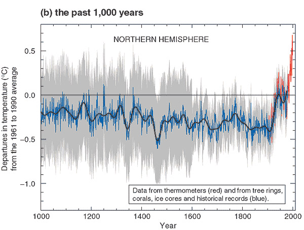
2_6_2 -1000 -> 1999
data source:
IPCC AR3, Third Assessment Report_climate change 2001:the science basis
chapter_Summary for Policymakers
Fig. 1b
IPCC AR3, Third Assessment Report_climate change 2001:the science basis
chapter_Summary for Policymakers
Fig. 1b
Millennial Northern Hemisphere (NH) temperature reconstruction (blue) and instrumental data (red) from ade 1000 to 1999, adapted
from Mann et al. (1999).
Smoother version of NH series (black), linear trend from AD 1000 to 1850 (purple-dashed) and two standard error limits (grey shaded) are shown.
Over both the last 140 years and 100 years, the best estimate is that the global average surface temperature has increased by 0.6 ± 0.2°C.
Smoother version of NH series (black), linear trend from AD 1000 to 1850 (purple-dashed) and two standard error limits (grey shaded) are shown.
Over both the last 140 years and 100 years, the best estimate is that the global average surface temperature has increased by 0.6 ± 0.2°C.
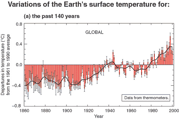
2_6_3 1860 -> 2000
data source:
IPCC AR3, Third Assessment Report_climate change 2001:the science basis
chapter_Summary for Policymakers
Fig. 1a
IPCC AR3, Third Assessment Report_climate change 2001:the science basis
chapter_Summary for Policymakers
Fig. 1a
Smoothed annual anomalies of combined land-surface air and sea surface temperatures (°C), 1861 to 2000, relative to 1961 to 1990, for the (c) Globe.
2_7 PNAS
Proceedings of the National Academy of Sciences
is the official scientific journal of the National Academy of Sciences,
is the official scientific journal of the National Academy of Sciences,
2_7_1 -22.000 -> 2000
data source:
Hengyu Liu et al., Pnas, 2014
PNAS vol. 111 no. 34 > Zhengyu Liu, E3501–E3505
The Holocene temperature conundrum
Fig. 1
Hengyu Liu et al., Pnas, 2014
PNAS vol. 111 no. 34 > Zhengyu Liu, E3501–E3505
The Holocene temperature conundrum
Fig. 1
Evolution of the global surface temperature of the last 22 ka:
the reconstructions of M13 (1) (blue) after 11.3 ka and by Shakun et al. (11) (cyan) before 6.5 ka, the model annual mean temperature averaged over the global grid points (black), and the model seasonally biased temperature averaged over the proxy sites (red).
the reconstructions of M13 (1) (blue) after 11.3 ka and by Shakun et al. (11) (cyan) before 6.5 ka, the model annual mean temperature averaged over the global grid points (black), and the model seasonally biased temperature averaged over the proxy sites (red).

1
INFO
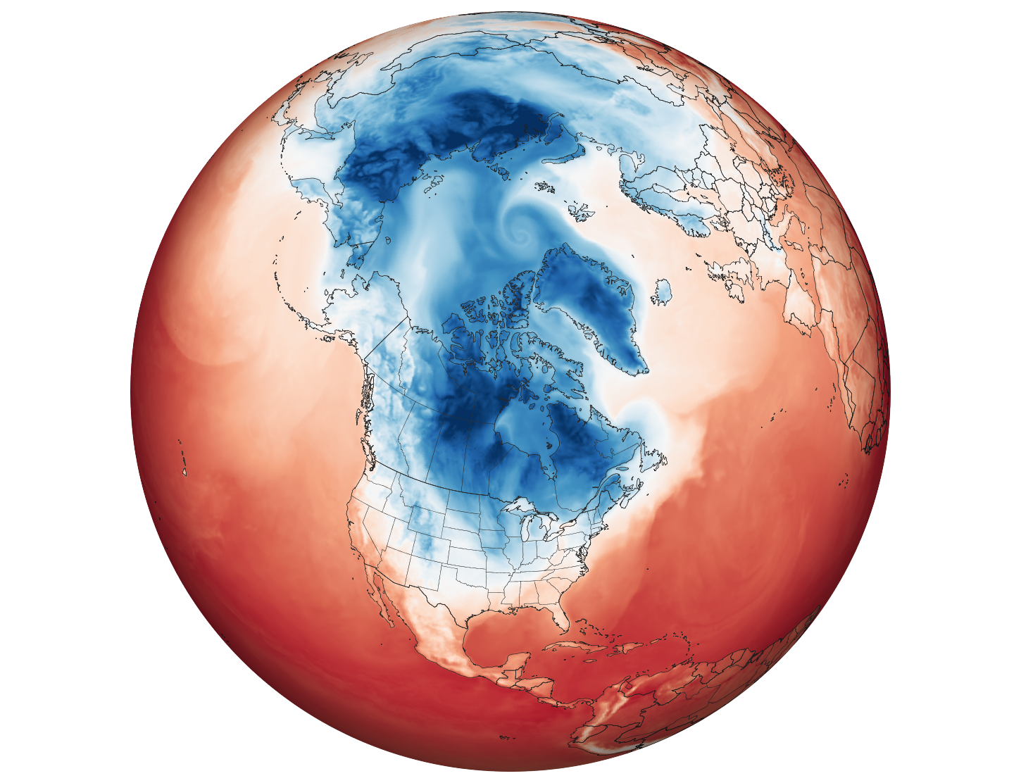
1_0 polar vortex
Normally, the olarVortxe swirls around the Arctic, trapping cold air near the Pole. Recently, this pressure system has been less stable, spilling colder air south & bringing record-low temperatures to parts of the continental U.S.
2019 29 01, Nasa
2019 29 01, Nasa
https://twitter.com/NASAEarth/status/1090674002576711680/photo/1
LINK --> gaya / jet stream
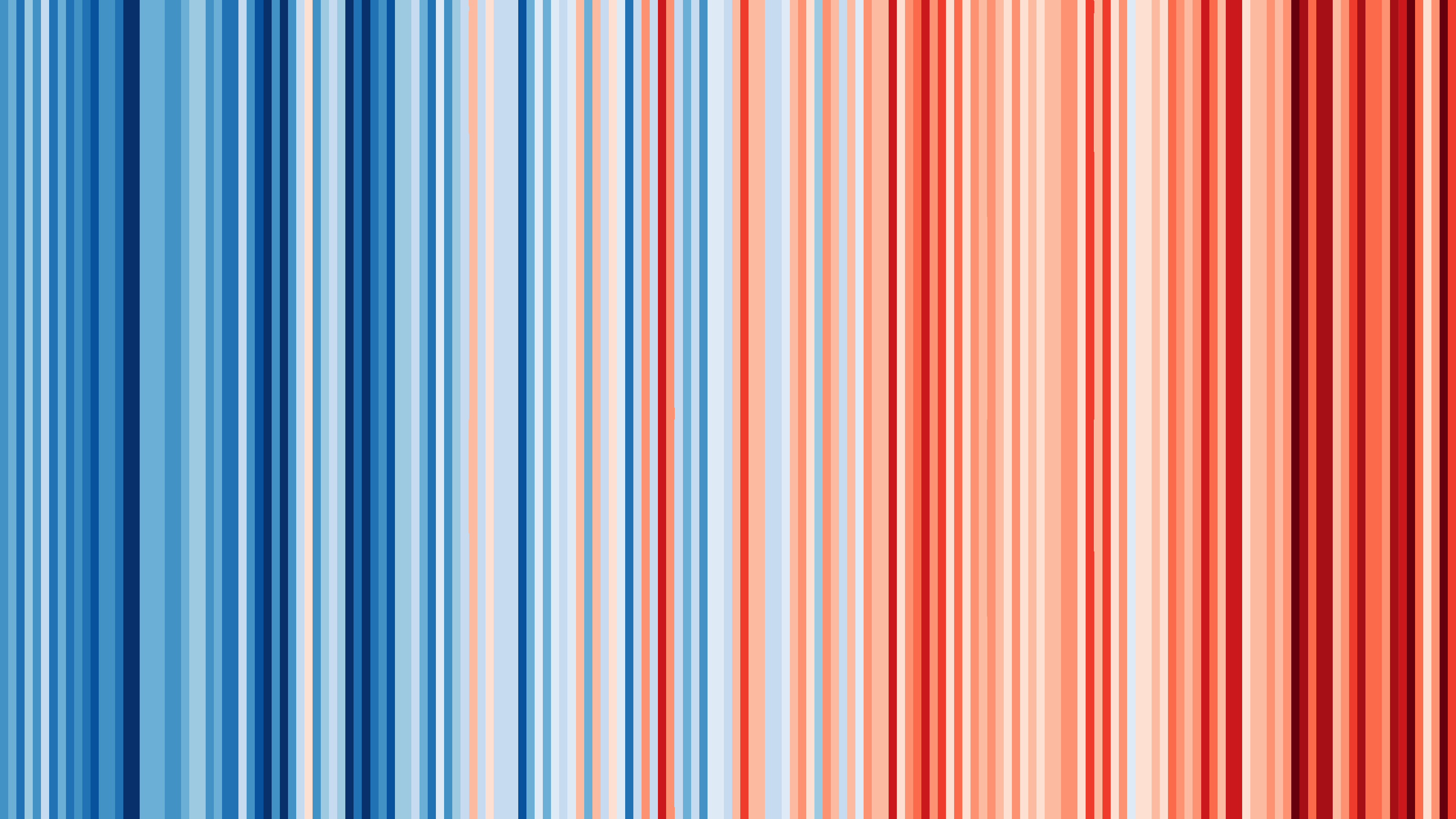
1_1.1 WORLD ann. temp. 1850 - 2017
Annual global temperatures from 1850-2017
temperature range color scale: 1.35°C
visualisation: Ed Hawkins
[Climate scientist in the National Centre for Atmospheric Science (NCAS) at the University of Reading. IPCC AR5 Contributing Author.]
data source:
Morice, C. P., J. J. Kennedy, N. A. Rayner, and P. D. Jones (2012),
Quantifying uncertainties in global and regional temperature change using an ensemble of observational estimates:
The HadCRUT4 dataset, J. Geophys. Res., 117, D08101, doi:10.1029/2011JD017187.

1_1.2 TORONTO ann. temp 1841-2017
temperature range color scale 5.5°C
[5.5°C - 11.0°C - dark blue to dark red]
[5.5°C - 11.0°C - dark blue to dark red]
1_1.2 GERMANY ann. temp 1881-2017
temperature range color scale 3.7°C
[6.6°C - 10.3°C - dark blue to dark red]
[6.6°C - 10.3°C - dark blue to dark red]
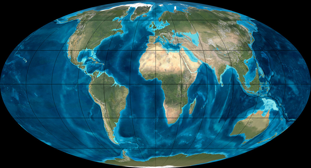
1_2 LAND + OCEAN tempertaure
global average tempertaure: composed of:
ocean tempertature [glob.aver.]
land temperature [glob.aver.]
"The area of the oceans remains cooler, than over land,
in a scenario [projection/simulation] where we have a global average temperature rise of eg. 4 degrees C, most land areas have warmed by more than 6 degrees C."
ocean tempertature [glob.aver.]
land temperature [glob.aver.]
"The area of the oceans remains cooler, than over land,
in a scenario [projection/simulation] where we have a global average temperature rise of eg. 4 degrees C, most land areas have warmed by more than 6 degrees C."
The Climate Crisis. Stefan Rahmstorf . 2013 10 05 . Earth101
citation_21m15s
citation_21m15s
1_3 C02 [/GG] cause warming
greenhouse effectf:
_Energy arrives from the sun in the form of visible light and ultraviolet radiation.
_The Earth then emits some of this energy as infrared radiation.
_Greenhouse gases in the atmosphere 'capture' some of this heat,
_ then re-emit it in all directions - including back to the Earth's surface.
Through this process, CO2 and other greenhouse gases keep the Earth’s surface 33°C warmer than it would be without them.
"So far, the average global temperature has gone up by about 0.8 degrees Csince 1880.
Two-thirds of the warming has occurred since 1975, at a rate of roughly 0.15-0.20°C per decade." [According to an ongoing temperature analysis conducted by scientists at NASA’s Goddard Institute for Space Studies (GISS)]
We have added 42% more CO2 since 1880.
data source:
Evans &Puckrin, AMESTOC, 2006
Measurements of the radiative surfaceforcing of climate
Fig. 1
Evans &Puckrin, AMESTOC, 2006
Measurements of the radiative surfaceforcing of climate
Fig. 1
Spectrum of the greenhouse radiation measured at the surface. Greenhouse effect from water vapour is filtered out, showing the contributions of other greenhouse gases.
1_4_1 SUN
is approximately ∼ 4.6 billion years [10 ↑ 9].
This age is estimated using computer models and nucleocosmochronology.
The result is consistent with the radiometric date of the oldest Solar System material, at 4.567 billion years ago.
This age is estimated using computer models and nucleocosmochronology.
The result is consistent with the radiometric date of the oldest Solar System material, at 4.567 billion years ago.

1_4_2 EARTH
is approximately 4.54 ± 0.05 billion years [10 ↑ 9].
This dating is based on evidence from radiometric age-dating of meteorite material and is consistent with the radiometric ages of the oldest-known terrestrial and lunar samples. [crystals of zircon from the Jack Hills of Western Australia are at least 4.4 billion years old.]
This dating is based on evidence from radiometric age-dating of meteorite material and is consistent with the radiometric ages of the oldest-known terrestrial and lunar samples. [crystals of zircon from the Jack Hills of Western Australia are at least 4.4 billion years old.]

1_5_1 MILANKOVIC cycles
Variations in eccentricity, axial tilt [obliquity], and precession of the Earth‘s orbit resultes in cyclical variation in the solar radiation reaching the Earth,
this orbital forcing strongly influences climatic patterns on Earth [alter the amount and location of solar radiation reaching the Earth]. This is known as solar forcing (an example of radiative forcing).
The Earth‘s orbit varies between nearly circular and mildly elliptical. Due to gravitational interactions with other bodies in the solar system, the Earth‘s rotation around its axis, and elliptical revolution around the Sun, evolve over time. They loosely combine into a 100,000-year cycle. [mathematicly described by Milutin Milanković, 1920‘s]
Khan Academy . Cosmology & Astronomy_.2011
SITE_https://www.khanacademy.org/science/cosmology-and-astronomy/earth-history-topic#earth-title-topic
SITE_https://www.khanacademy.org/science/cosmology-and-astronomy/earth-history-topic#earth-title-topic
1_5_2 Milankovitch cycles_ICE AGES
The episodic nature of the Earth‘s glacial and interglacial periods within the present Ice Age [Quaternary -2.500.000 -> now] have been caused primarily by cyclical changes in the Earth‘s circumnavigation of the Sun.
Variations in the Earth‘s eccentricity, axial tilt, and precession comprise the 3 dominant cycles.
Taken in unison, variations in these 3 cycles creates alterations in the seasonality of solar radiation reaching the Earth‘s surface.
These times of increased or decreased solar radiation directly influence the Earth‘s climate system, thus impacting the advance and retreat of Earth‘s glaciers.
CYCLES
01_Eccentricity
[100,000 years]
var. 0-5% [eccent.0,0006 - 0,058 ]
Earth‘s more and less elliptical orbit around the Sun.
NOW_low eccentricity [near circular]
[eccent 0,0167]
02_axial Tilt
[41.000 years]
var. 21.5 to 24.5 degrees.
less axial tilt = Sun‘s solar radiation is more evenly distributed between winter and summer + difference increases in radiation receipts between the equatorial and polar regions.
Axial tilt changes the strenght of the seasons over time.
NOW_middle of range [23.4 degrees]
[24.5 degree_-8700]
[23.4 degree_2017_now]
[21.5 degree_11.800]
03a_axial Precession
[23.000 years]
var. pointing at the North Star / at Vega
Earth‘s slow wobble as it spins on axis.
Earth tilts towards or away from the sun a little bit earlier or later every year.
03b_apsidal Precession
[112.000 years]
the orbital ellipse itself precesses in space completing a full cycle [primarily through interactions with Jupiter and Saturn]
01_Eccentricity[100,000 years]

02_axial Tilt [41.000 years]

03a_axial Precession[23.000 years]

03b_apsidal Precession [112.000 years]

1_6 ICE AGES
We are living now in the QUATERNARY Ice Age,
in the HOLOCENE interglacial period.
Glacials and Interglacials alter in a period of about 100.000 years. [ in the last mio of years]
--> Milankovic Cycles [describe cyclical changes in the Earth's circumnavigation of the Sun -> earth gets different quantities of energy]
Within ice ages, there exist periods of more severe glacial conditions = glacial periods, and more temperate = interglacial periods.
The Earth is currently in such an interglacial period of the Quaternary Ice Age.
The last glacial period of the Quaternary has ended approximately 11,700 years ago with the star of a interglacial period the HOLOCENE.
ICE AGES
06_QUATERNARY
[-2.500.000 ->]
04_Karoo
[-360.000.000 -> -260.000.000]
03_Andean-Saharan
[-450.000.000 -> -420.000.000]
02_Cryogenian
[-720.000.000 -> -635.000.000]
01_Huronian
[-2.450.000.000 - > -2.100.000.000]
06_QUATERNARY [-2.500.000 ->]
GALCIALS / INTER GLACIALS
[the nord european names]
HOLOCENE [-11.500 -> now]
_INTERGLACIAL
Weichselian [-110.000 -> -11.5000] _GLACIAL [last “ice age”]
Eemian [-130.000 -> -115.000]
_INTERGLACIAL
Saalian [-200.000 -> -130.0000]
_GLACIAL
Holstein [-424.000 -> -374.000]
_INTERGLACIAL
Elsterian [-478.000 -> - 424.0000]
_GLACIAL
x [-563.000 -> - 533.000 -> -476.000]
_INTERGLACIAL
Menapian [-676.000 -> -621.000] _GLACIAL

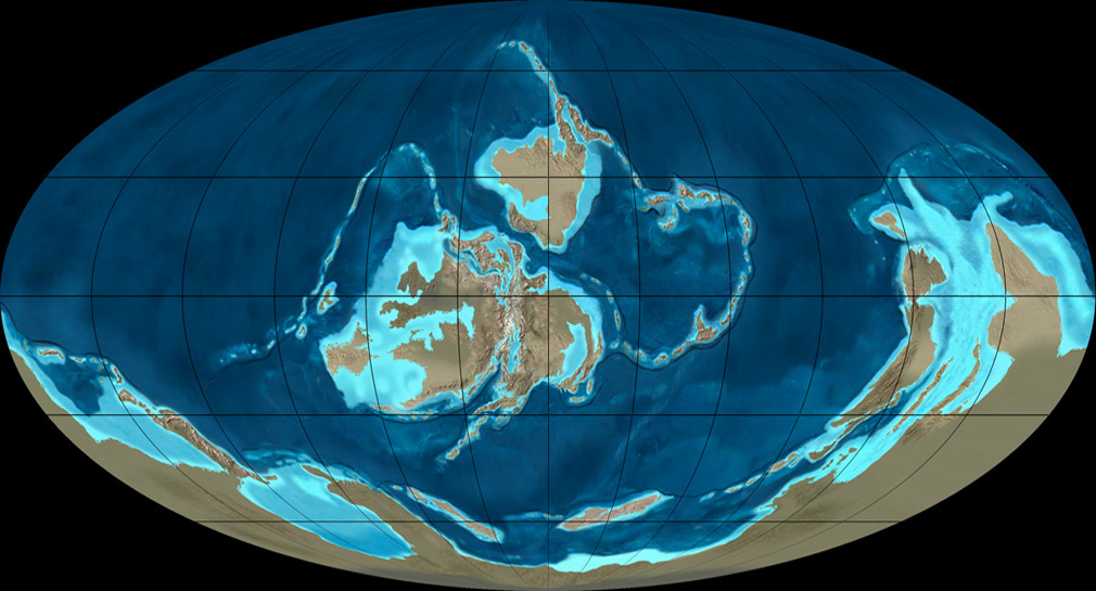
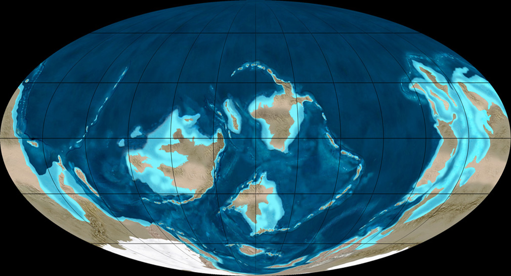
Earth at the last glacial maximum [WEICHSELIAN] of the current ice age. [Thomas J. Crowley , Global Biogeochemical Cycles, Vol. 9, 1995, pp. 377-389]
1_7 geological periods
01_EON_PROTerozoic
3 ERAs/
10 geologic PERIODs
2.500.000.000 -> 541.000.000
02_EON_PHANerozoic
3 ERAs/
12 geological PERIODs
541.000.000 -> 0
3 ERAs/
10 geologic PERIODs
2.500.000.000 -> 541.000.000
02_EON_PHANerozoic
3 ERAs/
12 geological PERIODs
541.000.000 -> 0
1_6_1 02_EON_PHANerozoic
02.3.3 Quaternary
[2.588.000 –>
0]
0]
02.3.2 Neogene
[23.000.000 –> 2.588.000]
02.3.1 Paleogene
[66.000.000 –> 23.000.000]
02.2.3 Cretaceous
[145.500.000 –> 66.000.000]
02.2.2 Jurassic
[20.100.000 –> 145.500.000]
02.2.1 Triassic
[252.000.000 –> 20.100.000]
02.1.6 Permian
[300.000.000 –> 252.000.000]
02.1.5 Carboniferous
[359.000.000 –> 300.000.000]
02.1.4 Devonian
[419.000.000 –> 359.000.000]
02.1.3 Silurian
[443.000.000 –> 419.000.000]
02.1.2 Ordovician
[541.000.000 –> 443.000.000]
02.1.1 Cambrian
[485.000.000 –> 541.000.000]
July 3rd, 2019